While we have taken steps to ensure the accuracy of this Internet version of the document, it is not the official version. Please refer to the official version in the FR publication, which appears on the Government Printing Office’s electronic CFR website
Method 203A – Visual Determination of Opacity of Emissions from Stationary Sources for Time-Averaged Regulations
1.0 Scope and Application
What is Method 203A?
Method 203A is an example test method suitable for State Implementation Plans (SIP) and is applicable to the determination of the opacity of emissions from sources of visible emissions for time-averaged regulations. A time-averaged regulation is any regulation that requires averaging visible emission data to determine the opacity of visible emissions over a specific time period.
Method 203A is virtually identical to EPA’s Method 9 of 40 CFR Part 60, Appendix A, except for the data-reduction procedures, which provide for averaging times other than 6 minutes.
Therefore, using Method 203A with a 6-minute averaging time would be the same as following EPA Method 9. The certification procedures for this method are identical to those provided in Method 9 and are provided here, in full, for clarity and convenience. An example visible emission observation form and instructions for its use can be found in reference 7 of Section 17 of Method 9.
2.0 Summary of Method
The opacity of emissions from sources of visible emissions is determined visually by an observer certified according to the procedures in Section 10 of this method. Readings taken every 15 seconds are averaged over a time period specified in the applicable regulation ranging from 2 minutes to 6 minutes.
3.0 Definitions [Reserved]
4.0 Interferences [Reserved]
5.0 Safety [Reserved]
6.1 Equipment and Supplies
What equipment and supplies are needed?
6.2 Stop Watch. Two watches are required that provide a continuous display of time to the nearest second.
6.3 Compass (optional). A compass is useful for determining the direction of the emission point from the spot where the visible emissions (VE) observer stands and for determining the wind direction at the source. For accurate readings, the compass should be magnetic with resolution better than 10 degrees. It is suggested that the compass be jewel-mounted and liquid-filled to dampen the needle swing; map reading compasses are excellent.
6.4 Range Finder (optional). Range finders determine distances from the observer to the emission point. The instrument should measure a distance of 1000 meters with a minimum accuracy of ±10 percent.
6.5 Abney Level (optional). This device for determining the vertical viewing angle should measure within 5 degrees.
6.6 Sling Psychrometer (optional). In case of the formation of a steam plume, a wet- and dry- bulb thermometer, accurate to 0.5°C, are mounted on a sturdy assembly and swung rapidly in the air in order to determine the relative humidity.
6.7 Binoculars (optional). Binoculars are recommended to help identify stacks and to characterize the plume. An 8 x 50 or 10 x 50 magnification, color-corrected coated lenses and rectilinear field of view is recommended.
6.8 Camera (optional). A camera is often used to document the emissions before and after the actual opacity determination.
6.9 Safety Equipment. The following safety equipment, which should be approved by the Occupational Safety and Health Association (OSHA), is recommended: orange or yellow hard hat, eye and ear protection, and steel-toed safety boots.
6.10 Clipboard and Accessories (optional). A clipboard, several ball-point pens (black ink recommended), a rubber band, and several visible emission observation forms facilitate documentation.
7.0 Reagents and Standards (Reserved]
8.1 Sample Collection, Preservation, Storage, and Transport
What is the Test Procedure?
An observer qualified in accordance with Section 10 of this method must use the following procedures to visually determine the opacity of emissions from stationary sources.
8.2 Procedure for Emissions from Stacks. These procedures are applicable for visually determining the opacity of stack emissions by a qualified observer.
8.2.1 Position. You must stand at a distance sufficient to provide a clear view of the emissions with the sun oriented in the 140-degree sector to your back. Consistent with maintaining the above requirement as much as possible, you must make opacity observations from a position such that the line of vision is approximately perpendicular to the plume direction, and when observing opacity of emissions from rectangular outlets (e.g., roof monitors, open baghouses, non-circular stacks), approximately perpendicular to the longer axis of the outlet. You should not include more than one plume in the line of sight at a time when multiple plumes are involved and, in any case, make opacity observations with the line of sight perpendicular to the longer axis of such a set of multiple stacks (e.g., stub stacks on baghouses).
8.2.2 Field Records. You must record the name of the plant, emission location, type of facility, observer’s name and affiliation, a sketch of the observer’s position relative to the source, and the date on a field data sheet. An example visible emission observation form can be found in reference 7 of Section 17 of this method. You must record the time, estimated distance to the emission location, approximate wind direction, estimated wind speed, description of the sky condition (presence and color of clouds), and plume background on the field data sheet at the time opacity readings are initiated and completed.
8.2.3 Observations. You must make opacity observations at the point of greatest opacity in that portion of the plume where condensed water vapor is not present. Do not look continuously at the plume but, instead, observe the plume momentarily at 15-second intervals.
8.2.3.1 Attached Steam Plumes. When condensed water vapor is present within the plume as it emerges from the emission outlet, you must make opacity observations beyond the point in the plume at which condensed water vapor is no longer visible. You must record the approximate distance from the emission outlet to the point in the plume at which the observations are made.
8.2.3.2 Detached Steam Plumes. When water vapor in the plume condenses and becomes visible at a distinct distance from the emission outlet, you must make the opacity observation at the emission outlet prior to the condensation of water vapor and the formation of the steam plume.
8.2 Recording Observations. You must record the opacity observations to the nearest 5 percent every 15 seconds on an observational record sheet such as the example visible emission observation form in reference 7 of Section 17 of this method. Each observation recorded represents the average opacity of emissions for a 15-second period. The overall length of time for which observations are recorded must be appropriate to the averaging time specified in the applicable regulation.
9.0 Quality Control [Reserved]
10.1 Calibration and Standardization
10.2 What are the Certification Requirements? To receive certification as a qualified observer, you must be trained and knowledgeable on the procedures in Section 8.0 of this method, be tested and demonstrate the ability to assign opacity readings in 5 percent increments to 25 different black plumes and 25 different white plumes, with an error not to exceed 15 percent opacity on any one reading and an average error not to exceed 7.5 percent opacity in each category. You must be tested according to the procedures described in Section 10.2 of this method. Any smoke generator used pursuant to Section 10.2 of this method must be equipped with a smoke meter which meets the requirements of Section 10.3 of this method. Certification tests that do not meet the requirements of Sections 10.2 and 10.3 of this method are not valid.
The certification must be valid for a period of 6 months, and after each 6-month period, the qualification procedures must be repeated by an observer in order to retain certification.
10.3 What is the Certification Procedure? The certification test consists of showing the candidate a complete run of 50 plumes, 25 black plumes and 25 white plumes, generated by a smoke generator. Plumes must be presented in random order within each set of 25 black and 25 white plumes. The candidate assigns an opacity value to each plume and records the observation on a suitable form. At the completion of each run of 50 readings, the score of the candidate is determined. If a candidate fails to qualify, the complete run of 50 readings must be repeated in any retest. The smoke test may be administered as part of a smoke school or training program, and may be preceded by training or familiarization runs of the smoke generator during which candidates are shown black and white plumes of known opacity.
10.4 Smoke Generator.
10.4.1 What are the Smoke Generator Specifications? Any smoke generator used for the purpose of Section 10.2 of this method must be equipped with a smoke meter installed to measure opacity across the diameter of the smoke generator stack. The smoke meter output must display in-stack opacity, based upon a path length equal to the stack exit diameter on a full 0 to 100 percent chart recorder scale. The smoke meter optical design and performance must meet the specifications shown in Table 203A–1 of this method. The smoke meter must be calibrated as prescribed in Section 10.3.2 of this method prior to conducting each smoke reading test. At the completion of each test, the zero and span drift must be checked and, if the drift exceeds ±1 percent opacity, the condition must be corrected prior to conducting any subsequent test runs. The smoke meter must be demonstrated at the time of installation to meet the specifications listed in Table 203A–1 of this method. This demonstration must be repeated following any subsequent repair or replacement of the photocell or associated electronic circuitry including the chart recorder or output meter, or every 6 months, whichever occurs first.
10.4.2 How is the Smoke Meter Calibrated? The smoke meter is calibrated after allowing a minimum of 30 minutes warm-up by alternately producing simulated opacity of 0 percent and 100 percent. When a stable response at 0 percent or 100 percent is noted, the smoke meter is adjusted to produce an output of 0 percent or 100 percent, as appropriate. This calibration must be repeated until stable 0 percent and 100 percent readings are produced without adjustment. Simulated 0 percent and 100 percent opacity values may be produced by alternately switching the power to the light source on and off while the smoke generator is not producing smoke.
10.4.3 How is the Smoke Meter Evaluated? The smoke meter design and performance are to be evaluated as follows:
10.4.3.1 Light Source. You must verify from manufacturer’s data and from voltage measurements made at the lamp, as installed, that the lamp is operated within 5 percent of the nominal rated voltage.
10.4.3.2 Spectral Response of the Photocell. You must verify from manufacturer’s data that the photocell has a photopic response; i.e. , the spectral sensitivity of the cell must closely approximate the standard spectral-luminosity curve for photopic vision which is referenced in (b) of Table 203A–1 of this method.
10.4.3.3 Angle of View. You must check construction geometry to ensure that the total angle of view of the smoke plume, as seen by the photocell, does not exceed 15 degrees. Calculate the total angle of view as follows:
φv= 2 tan−1(d/2L) Where:
φv= Total angle of view
d = The photocell diameter + the diameter of the limiting aperture L = Distance from the photocell to the limiting aperture.
The limiting aperture is the point in the path between the photocell and the smoke plume where the angle of view is most restricted. In smoke generator smoke meters, this is normally an orifice plate.
10.4.3.4 Angle of Projection. You must check construction geometry to ensure that the total angle of projection of the lamp on the smoke plume does not exceed 15 degrees. Calculate the total angle of projection as follows:
φp= 2 tan−1(d/2L) Where:
φp= Total angle of projection
d = The sum of the length of the lamp filament + the diameter of the limiting aperture L = The distance from the lamp to the limiting aperture.
10.4.3.5 Calibration Error. Using neutral-density filters of known opacity, you must check the error between the actual response and the theoretical linear response of the smoke meter. This check is accomplished by first calibrating the smoke meter according to Section 10.3.2 of this method and then inserting a series of three neutral-density filters of nominal opacity of 20, 50, and 75 percent in the smoke meter path length. Use filters calibrated within 2 percent. Care should be taken when inserting the filters to prevent stray light from affecting the meter. Make a total of five non-consecutive readings for each filter. The maximum opacity error on any one reading shall be ±3 percent.
10.4.3.6 Zero and Span Drift. Determine the zero and span drift by calibrating and operating the smoke generator in a normal manner over a 1-hour period. The drift is measured by checking the zero and span at the end of this period.
10.4.3.7 Response Time. Determine the response time by producing the series of five simulated 0 percent and 100 percent opacity values and observing the time required to reach stable response. Opacity values of 0 percent and 100 percent may be simulated by alternately switching the power to the light source off and on while the smoke generator is not operating.
11.0 Analytical Procedures [Reserved]
12.1 Data Analysis and Calculations
12.2 Time-Averaged Regulations. A set of observations is composed of an appropriate number of consecutive observations determined by the averaging time specified ( i.e. , 8 observations for a two minute average). Divide the recorded observations into sets of appropriate time lengths for the specified averaging time. Sets must consist of consecutive observations; however, observations immediately preceding and following interrupted observations shall be deemed consecutive. Sets need not be consecutive in time and in no case shall two sets overlap. For each set of observations, calculate the average opacity by summing the opacity readings taken over the appropriate time period and dividing by the number of readings. For example, for a 2-minute average, eight consecutive readings would be averaged by adding the eight readings and dividing by eight.
13.1 Method Performance
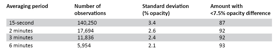
13.2 Time-averaging Performances. The accuracy of test procedures for time-averaged regulations was evaluated through field studies that compare the opacity readings to a transmissometer. Analysis of these data shows that, as the time interval for averaging increases, the positive error decreases. For example, over a 2-minute time period, 90 percent of the results underestimated opacity or overestimated opacity by less than 9.5 percent opacity, while over a 6- minute time period, 90 percent of the data have less than a 7.5 percent positive error. Overall, the field studies demonstrated a negative bias. Over a 2-minute time period, 57 percent of the data have zero or negative error, and over a 6-minute time period, 58 percent of the data have zero or negative error. This means that observers are more likely to assign opacity values that are below, rather than above, the actual opacity value. Consequently, a larger percentage of noncompliance periods will be reported as compliant periods rather than compliant periods reported as violations. Table 203A–2 highlights the precision data results from the June 1985 report: “Opacity Errors for Averaging and Non Averaging Data Reduction and Reporting Techniques.”
14.0 Pollution Prevention [Reserved]
15.0 Waste Management [Reserved]
16.0 Alternative Procedures [Reserved]
17.0 References
- U.S. Environmental Protection Agency. Standards of Performance for New Stationary Sources; Appendix A; Method 9 for Visual Determination of the Opacity of Emissions from Stationary Sources. Final Rule. 39 FR 219. Washington, DC. U.S. Government Printing Office. November 12, 1974.
- Office of Air and Radiation. “Quality Assurance Guideline for Visible Emission Training Programs.” EPA–600/S4–83–011. Quality Assurance Division. Research Triangle Park, NC. May 1982.
- Office of Research and Development. “Method 9—Visible Determination of the Opacity of Emissions from Stationary Sources.” February 1984. Quality Assurance Handbook for Air Pollution Measurement Systems. Volume III, Section 3.1.2. Stationary Source Specific Methods. EPA–600–4–77–027b. August 1977. Office of Research and Development Publications, 26 West Clair Street, Cincinnati, OH.
- Office of Air Quality Planning and Standards. “Opacity Error for Averaging and Non- averaging Data Reduction and Reporting Techniques.” Final Report–SR–1–6–85. Emission Measurement Branch, Research Triangle Park, NC. June 1985.
- U.S. Environmental Protection Agency. Preparation, Adoption, and Submittal of State Implementation Plans. Methods for Measurement of PM10Emissions from Stationary Sources. Final Rule.Federal Register.Washington, DC. U.S. Government Printing Office. Volume 55, No. 74. Pages 14246–14279. April 17, 1990.
- Office of Air Quality Planning and Standards. “Collaborative Study of Opacity Observations of Fugitive Emissions from Unpaved Roads by Certified Observers.” Emission Measurement Branch, Research Triangle Park, NC. October 1986.
- Office of Air Quality Planning and Standards. “Field Data Forms and Instructions for EPA Methods 203A, 203B, and 203C.” EPA 455/R–93–005. Stationary Source Compliance Division, Washington, DC, June 1993.
18.0 Tables, Diagrams, Flowcharts, and Validation Data
Table 203A–1—Smoke Meter Design and Performance Specifications
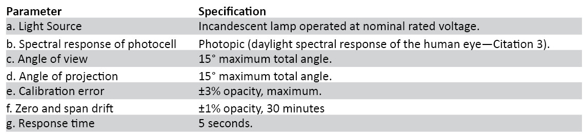
Table 203A–2—Precision Between Observers: Opacity Averaging